Converging Diverging Nozzle

Source Code

Instructions

Introduction
The purpose of this applet is to simulate the operation of a converging-diverging nozzle, perhaps the most important and basic piece of engineering hardware associated with propulsion and the high speed flow of gases. This device was invented by Carl de Laval toward the end of the l9th century and is thus often referred to as the 'de Laval' nozzle. This applet is intended to help students of compressible aerodynamics visualize the flow through this type of nozzle at a range of conditions.

Technical Background
The usual configuration for a converging diverging (CD) nozzle is shown in the figure. Gas flows through the nozzle from a region of high pressure (usually referred to as the chamber) to one of low pressure (referred to as the ambient or tank). The chamber is usually big enough so that any flow velocities here are negligible. The pressure here is denoted by the symbol p_c. Gas flows from the chamber into the converging portion of the nozzle, past the throat, through the diverging portion and then exhausts into the ambient as a jet. The pressure of the ambient is referred to as the 'back pressure' and given the symbol p_b.

A simple example
To get a basic feel for the behavior of the nozzle imagine performing the simple experiment shown in figure 2. Here we use a converging diverging nozzle to connect two air cylinders. Cylinder A contains air at high pressure, and takes the place of the chamber. The CD nozzle exhausts this air into cylinder B, which takes the place of the tank.

Imagine you are controlling the pressure in cylinder B, and measuring the resulting mass flow rate through the nozzle. You may expect that the lower you make the pressure in B the more mass flow you'll get through the nozzle. This is true, but only up to a point. If you lower the back pressure enough you come to a place where the flow rate suddenly stops increasing all together and it doesn't matter how much lower you make the back pressure (even if you make it a vacuum) you can't get any more mass flow out of the nozzle. We say that the nozzle has become 'choked'. You could delay this behavior by making the nozzle throat bigger (e.g. grey line) but eventually the same thing would happen. The nozzle will become choked even if you eliminated the throat altogether and just had a converging nozzle.

The reason for this behavior has to do with the way the flows behave at Mach 1, i.e. when the flow speed reaches the speed of sound. In a steady internal flow (like a nozzle) the Mach number can only reach 1 at a minimum in the cross-sectional area. When the nozzle isn't choked, the flow through it is entirely subsonic and, if you lower the back pressure a little, the flow goes faster and the flow rate increases. As you lower the back pressure further the flow speed at the throat eventually reaches the speed of sound (Mach 1). Any further lowering of the back pressure can't accelerate the flow through the nozzle any more, because that would entail moving the point where M=1 away from the throat where the area is a minimum, and so the flow gets stuck. The flow pattern downstream of the nozzle (in the diverging section and jet) can still change if you lower the back pressure further, but the mass flow rate is now fixed because the flow in the throat (and for that matter in the entire converging section) is now fixed too.

The changes in the flow pattern after the nozzle has become choked are not very important in our thought experiment because they don't change the mass flow rate. They are, however, very important however if you were using this nozzle to accelerate the flow out of a jet engine or rocket and create propulsion, or if you just want to understand how high-speed flows work.

The flow pattern
Figure 3a shows the flow through the nozzle when it is completely subsonic (i.e. the nozzle isn't choked). The flow accelerates out of the chamber through the converging section, reaching its maximum (subsonic) speed at the throat. The flow then decelerates through the diverging section and exhausts into the ambient as a subsonic jet. Lowering the back pressure in this state increases the flow speed everywhere in the nozzle.

Lower it far enough and we eventually get to the situation shown in figure 3b. The flow pattern is exactly the same as in subsonic flow, except that the flow speed at the throat has just reached Mach 1. Flow through the nozzle is now choked since further reductions in the back pressure can't move the point of M=1 away from the throat. However, the flow pattern in the diverging section does change as you lower the back pressure further.

As p_b is lowered below that needed to just choke the flow a region of supersonic flow forms just downstream of the throat. Unlike a subsonic flow, the supersonic flow accelerates as the area gets bigger. This region of supersonic acceleration is terminated by a normal shock wave. The shock wave produces a near-instantaneous deceleration of the flow to subsonic speed. This subsonic flow then decelerates through the remainder of the diverging section and exhausts as a subsonic jet. In this regime if you lower or raise the back pressure you increase or decrease the length of supersonic flow in the diverging section before the shock wave.

If you lower p_b enough you can extend the supersonic region all the way down the nozzle until the shock is sitting at the nozzle exit (figure 3d). Because you have a very long region of acceleration (the entire nozzle length) in this case the flow speed just before the shock will be very large in this case. However, after the shock the flow in the jet will still be subsonic.

Lowering the back pressure further causes the shock to bend out into the jet (figure 3e), and a complex pattern of shocks and reflections is set up in the jet which will now involve a mixture of subsonic and supersonic flow, or (if the back pressure is low enough) just supersonic flow. Because the shock is no longer perpendicular to the flow near the nozzle walls, it deflects it inward as it leaves the exit producing an initially contracting jet. We refer to this as overexpanded flow because in this case the pressure at the nozzle exit is lower than that in the ambient (the back pressure)- i.e. the flow has been expanded by the nozzle to much.

A further lowering of the back pressure changes and weakens the wave pattern in the jet. Eventually we will have lowered the back pressure enough so that it is now equal to the pressure at the nozzle exit. In this case, the waves in the jet disappear altogether (figure 3f), and the jet will be uniformly supersonic. This situation, since it is often desirable, is referred to as the 'design condition'.

Finally, if we lower the back pressure even further we will create a new imbalance between the exit and back pressures (exit pressure greater than back pressure), figure 3g. In this situation (called 'underexpanded') what we call expansion waves (that produce gradual turning and acceleration in the jet) form at the nozzle exit, initially turning the flow at the jet edges outward in a plume and setting up a different type of complex wave pattern.

The pressure distribution in the nozzle
A plot of the pressure distribution along the nozzle (figure 4) provides a good way of summarizing its behavior. To understand how the pressure behaves you have to remember only a few basic rules

When the flow accelerates (sub or supersonically) the pressure drops
The pressure rises instantaneously across a shock
The pressure throughout the jet is always the same as the ambient (i.e. the back pressure) unless the jet is supersonic and there are shocks or expansion waves in the jet to produce pressure differences.
The pressure falls across an expansion wave.

The labels on figure 4 indicate the back pressure and pressure distribution for each of the flow regimes illustrated in figure 3. Notice how, once the flow is choked, the pressure distribution in the converging section doesn't change with the back pressure at all.

Operating Instructions for the applet.
All of the above description is quite a lot to understand and remember without actually having a converging diverging nozzle to look at. This is the ideal of the applet - to give you a model of a nozzle that you can play around with and get experience of.

To start the program, go to the applet page and press the button labeled 'Start!' a window like that shown below will appear.

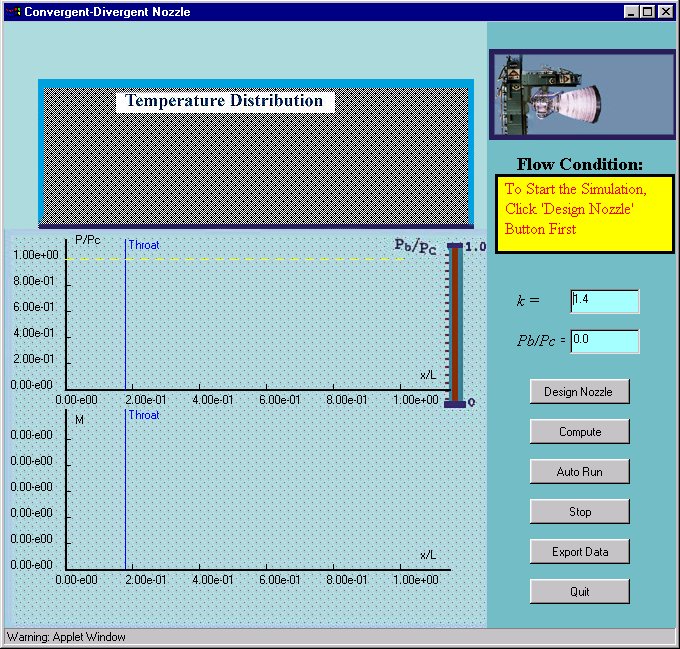
On the left hand side of the window there are three panels used for plotting the flow conditions in the nozzle. The top panel, shaded gray, is used to show the shape of the nozzle and a color contour map of the temperature distribution within it. Initially this region will be blank, note that the temperature distribution behaves qualitatively like the pressure distribution. The middle panel is used to display the pressure (vertical axis) as a function of distance down the nozzle (horizontal axis), and the lower panel displays the Mach number (flow speed over local speed of sound) as a function of distance. When results are displayed, the horizontal axes of these three panels all line up so the association between features on the different plots can easily be observed. On the top right of the applet window a graphic is displayed showing an actual rocket nozzle in a test stand. Below this is a yellow information panel, and then text areas where you can enter k the ratio of specific heats for the gas in the nozzle, and Pb/Pc the pressure ratio that is driving the flow through the nozzle. Below are a series of six buttons used to control the actions of the applet.

To begin press the 'Design Nozzle' button, which should bring up a window like that shown in the figure. On the right of the window there is a text area that allows you to enter the ratio of the exit area (Ae) to the throat area (At). This must be greater than 1. The larger the ratio, the higher the Mach number of the flow that your nozzle will produce (if you set this number very high, say >10) it may be difficult to see all the results clearly on the plots. Type in '4' and press the 'Set' button. The graph on the left shows the shape of the nozzle, chamber on the left, exit on the right. The program assumes you are dealing with an axisymmetric nozzle so, for example, your nozzle (with an area ratio of 4) will appear as having an exit with a diameter of twice that at the throat. You can change the shape of the diverging section by clicking the area shaded with '+' signs close to the line representing the diverging section. Note that you can't move the throat, or create a diverging section with a maximum in area - the program will warn you if either of these occurs. When you are satisfied with the shape, press the 'Done' button.

You can compute and display the flow through the nozzle in one of two ways. The most direct way is to enter a value for the back pressure in the text area labeled 'Pb/Pc'. Enter '0.5' and press the 'Compute' button. Almost instantaneously the results should be plotted as shown below.

The flow you have computed corresponds to case (c) in figure 3 above, i.e. flow with a shock in the nozzle (this is also stated in the yellow panel). On the top left of the frame a contour map of the flow temperature is plotted, normalized on the temperature in the chamber. Notice how the temperature falls as the flow accelerates up to and past the throat, and then suddenly rises in the shock wave. The center left plot shows the pressure distribution and beneath that is plotted the Mach number distribution. Notice how (of course) the Mach number is 1 at the throat in this case, and how the Mach number drops from super to subsonic across the shock wave. If you want you can access the numerical results of this calculation by pressing the 'Export data' button, copying out the numbers and pasting them into another application, like Excel, or Notepad.

The second way to compute the flow is the most useful if you want to see the whole range of phenomena present in the flow at different back pressures. To do this press the 'Auto Run' button. The program begins slowly lowers and raises the back pressure computing in small increments the entire flow and displaying the results. The net effect is an animation of what occurs in the nozzle as you raise and lower the back pressure. You can stop the animation at any time by pressing 'Stop'. To leave the applet you should press the 'Quit' button (pressing the 'X' at the top left hand corner of the frame doesn't work).

How the applet works.
The applet works by computing the flow using the one dimensional equations for the isentropic flow of a perfect gas, and the Rankine Hugoniot relations for normal shock waves in perfect gases. You can learn about these relations by reading, form example, Modern Compressible Flow, 2nd Edition, 1990, by John D. Anderson Jr. You can use the Compressible Aerodynamics Calculator to help you use these relations in your own calculations.

Run the Applet

Source Code

Current Applet Version 1.0. Last HTML/Applet update 1/3/01. Questions or comments please contact William J. Devenport